Data Collection

All the loyal3 stocks are all listed on a single page. Before you can look up individual daily stock prices to build your trading algorithm, you need to collect all available stocker tickers. The first thing to do is declare stock.listas a URL string. Next use read_html() so your R session will create an Internet session and collect all the html information on the page as an XML node set. The page CSS has an ID called “.company-name”. Use this as a parameter when calling html_nodes() to select only the XML data associated to this node. Lastly, use html_text()so the actual text values for the company names is collected.

stock.list<-'https://www.loyal3.com/stocks'
stocks<-read_html(stock.list)
stocks.names<-html_nodes(stocks,'.company-name')
stocks.names<-html_text(stocks.names)

To examine the stocks that are available on loyal3, you can print the stocks.names object to your console. This returns the company name as a text vector.

stocks.names 

In order to research the stock prices, you need to get the ticker symbol first. When you are on the loyal3 site, you can click on the company tile to load a page with a ticker symbol and other company information.

Using html_nodes() on stocks, you pull all nodes marked with an “a.” In HTML the <a> tag defines a hyperlink which is used to link form one page to another. Within the hyperlink tag, the “href” refers to the exact URL address. So html_attr() will extract the URL for ALL links on the page if you pass in “href”.

After doing some manual inspection, I found the 54th to 123rd links on the page represent the company pages I need in order to scrape the ticker information. The last line uses paste0() to concatenate the base URL string ’http://www.loyal3.com` to the specific company pages, like “/WALMART”. For example, http://www.loyal3.com/WALMART:

loyal.links<-html_nodes(stocks, "a")
loyal.links<-html_attr(loyal.links, "href")
stock.links<-paste0('http://www.loyal3.com',loyal.links[54:123])

On each of the company pages there is a description, a recent closing price and the ticker. All company pages are organized the same so the custom function get.ticker() can be used to extract the ticker symbol.

Within a company’s web page there is a table called “ticker-price”. The function will navigate to a company page, identify the appropriate table, extract the text with html_text(). Lastly, using sub() along with the regular expression ^([[:alpha:]]*).* and \\1 will retain all alphabetical characters. The result is that the any special characters, like $, and any numeric characters, like the closing price, are removed. As the function reads each of the 70 pages, it will only collect the stock ticker.

get.ticker<-function(url){
  x<-read_html(url)
  x<-html_node(x,'.ticker-price')
  x<-html_text(x)
  x<-sub("^([[:alpha:]]*).*", "\\1", x)
  return(x)
  } 

Armed with your custom function, use pblapply() to apply it to each of the stock.links which contain each company’s page. The resulting object, stock.tickers, is a list of individual stock tickers with each element corresponding to an individual company.

stock.tickers<-pblapply(stock.links,get.ticker)

One way to change a list of elements into a flat object is with do.call(). Here, you are applying rbind to row bind each list element into a single vector. Lastly, you create a data frame with the symbol and company name information.

stock.ticks<-do.call(rbind,stock.tickers)
stock.ticks<-data.frame(symbol=stock.ticks,name=stocks.names)

To be consistent in your analysis, you may want to limit the amount of historical information you gather on each stock. The Sys.Data() function will store a date object as year, month and then day. Using years with an integer is one way to subtract a specific amount of time from the start.date object.

start.date<-Sys.Date()
end.date<-Sys.Date()-years(3)

To get the Yahoo finance data, the date object has to be changed to simple character objects without a dash. Using the global substitution function gsub() on both start.date and end.date will change the class and simultaneously remove dashes. Within gsub(), pass in the character pattern to search for, then the replacement characters. In this case the replacing pattern is an empty character in between quotes. The last parameter is the object that gsub() will be applied to.

start.date<-gsub('-','', start.date)
end.date<-gsub('-','', end.date)

The TTR() function getYahooData() accepts a stock symbol, and a starting and ending date. The function returns a data frame that has time series information. Each row is a date and the columns contain information such as the “Open”, “High”, “Low” and “Closing” price for an equity. Since you are looking up multiple companies, you can use lapply() or pblapply(). Pass in the vector of company symbols, then the function, getYahooData(), and then the date information. The date objects are recycled parameters each time getYahooData() is applied to a stock symbol.

 stocks.ts<-pblapply(stock.ticks$symbol,getYahooData,end.date, start.date)

To make selecting the returned list, stocks.ts, easier to navigate you can add names to the list elements. Using names with the stocks.ts object declare the names as the original $symbol vector.

names(stocks.ts)<-stock.ticks$symbol

When working with large lists, I like to examine the resulting object to make sure the outcome is what I expected. Now that the elements have names, you can reference them directly. In this example, you are examining the first 6 rows for AMC Entertainment Holdings (AMC). Using head() on the list while referencing $AMC will return a portion of the time series for this stock:

head(stocks.ts$AMC)

Examining the Stock Data

When I listen to financial news commentators often refer to charts. Despite high frequency trading and active management performed by others, many small investors still refer to charts to gain insight. The time series object can be quickly displayed using plot. Pass in the list referring to the named element such as $AMC and then the column you want to display, here $Close.

plot(stocks.ts$AMZN$Close)

The preceding plot is static and not very interesting.

Let’s use a JavaScript library to make a chart you can explore. In this code snippet, you may observe the “%>%” or pipe operator. The pipe operator is a good way to write concise code. It forwards an object to the next function without forcing you to rewrite an object name like you did earlier in this post.

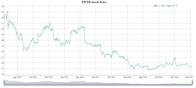
In this example, you create a dygraph referring to the Twitter stock, $TWTR, and then the column you want to plot, $Close. Within dygraph, main adds a title that is specified in between the quotes. Using the “%>%” this entire object is forwarded to the next function dyRangeSelector(). You can specify a default date range using c()with a start and end date string. The resulting HTML object is a dynamic time series for Twitter’s stock with a date slider at the bottom.

Remember, to change the equity displayed, change the ticker symbol in the stocks.ts list and then the graph title.

dygraph(stocks.ts$TWTR$Close, main = "TWTR Stock Price") %>%
  dyRangeSelector(dateWindow = c("2013-12-18", "2016-12-30"))